(Solved): Asap the subgraph of G obtained by adding the vertex y and the edge xy to T is again a tree in ...

Asap

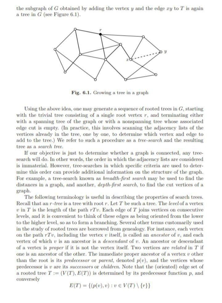
the subgraph of $$G$$ obtained by adding the vertex $$y$$ and the edge $$xy$$ to $$T$$ is again a tree in $$G$$ (see Figure 6.1). Fig. 6.1. Growing a tree in a graph Using the above idea, one may generate a sequence of rooted trees in $$G$$, starting with the trivial tree consisting of a single root vertex $$r$$, and terminating either with a spanning tree of the graph or with a nonspanning tree whose associated edge cut is empty. (In practice, this involves scanning the adjacency lists of the vertices already in the tree, one by one, to determine which vertex and edge to add to the tree.) We refer to such a procedure as a tree-search and the resulting tree as a search tree. If our objective is just to determine whether a graph is connected, any treesearch will do. In other words, the order in which the adjacency lists are considered is immaterial. However, tree-searches in which specific criteria are used to determine this order can provide additional information on the structure of the graph. For example, a tree-search known as breadth-first search may be used to find the distances in a graph, and another, depth-first search, to find the cut vertices of a graph. The following terminology is useful in describing the properties of search trees. Recall that an $$r$$-tree is a tree with root $$r$$. Let $$T$$ be such a tree. The level of a vertex $$v$$ in $$T$$ is the length of the path $$rTv$$. Each edge of $$T$$ joins vertices on consecutive levels, and it is convenient to think of these edges as being oriented from the lower to the higher level, so as to form a branching. Several other terms customarily used in the study of rooted trees are borrowed from genealogy. For instance, each vertex on the path $$rTv$$, including the vertex $$v$$ itself, is called an ancestor of $$v$$, and each vertex of which $$v$$ is an ancestor is a descendant of $$v$$. An ancestor or descendant of a vertex is proper if it is not the vertex itself. Two vertices are related in $$T$$ if one is an ancestor of the other. The immediate proper ancestor of a vertex $$v$$ other than the root is its predecessor or parent, denoted $$p(v)$$, and the vertices whose predecessor is $$v$$ are its successors or children. 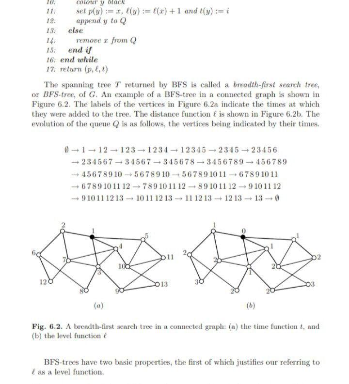Note that the (oriented) edge set of a rooted tree $$T:=(V(T),E(T))$$ is determined by its predecessor function $$p$$, and conversely $$E(T)=\{(p(v),v):v?V(T)\backslash \{r\}\}$$ 11: set $$p(y):=x,?(y):=?(x)+1$$ and $$t(y):=i$$ 12: append $$y$$ to $$Q$$ 13: else 14: remove $$x$$ from $$Q$$ 15: end if 16: end while 17: return $$(p,?,t)$$ The spanning tree $$T$$ returned by BFS is called a breadth-first search tree, or BFS-tree, of G. An example of a BFS-tree in a connected graph is shown in Figure 6.2. The labels of the vertices in Figure $$6.2\mathrm{a}$$ indicate the times at which they were added to the tree. The distance function $$?$$ is shown in Figure $$6.2\mathrm{b}$$. The evolution of the queue $$Q$$ is as follows, the vertices being indicated by their times. $$\begin{array}{rl}?& ?1?12?123?1234?12345?2345?23456\\ & ?234567?34567?345678?3456789?456789\\ & ?45678910?5678910?567891011?67891011\\ & ?6789101112?789101112?89101112?9101112\\ & ?910111213?10111213?111213?1213?13??\end{array}$$ $$(12)$$ (0) Fig. 6.2. A breadth-first search tree in a connected graph: (a) the time function $$t$$, and (b) the level function $$?$$ BFS-trees have two basic properties, the first of which justifies our referring to $$?$$ as a level function. 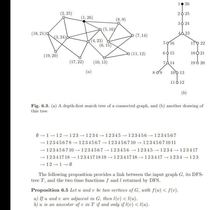$$(0)$$ Fig. 6.3. (a) A depth-first search tree of a connected graph, and (b) another drawing of this tree $$\begin{array}{rl}?& ?1?12?123?1234?12345?123456?1234567\\ & ?12345678?1234567?123456710?12345671011\\ & ?123456710?1234567?123456?12345?1234?123417\\ & ?12341718?1234171819?12341718?123417?1234?123\\ & ?12?1??\end{array}$$ The following proposition provides a link between the input graph $$G$$, its DFStree $$T$$, and the two time functions $$f$$ and $$l$$ returned by DFS. Proposition $$6.5$$ Let $$u$$ and $$v$$ be two vertices of $$G$$, with $$f(u)<f(v)$$. a) If $$u$$ and $$v$$ are adjacent in $$G$$, then $$l(v)<l(u)$$. b) $$u$$ is an ancestor of $$v$$ in $$T$$ if and only if $$l(v)<l(u)$$.