(Solved): Fourier series visualization Given x(t) in the figure below. Find the Fourier series for x(t). Writ ...

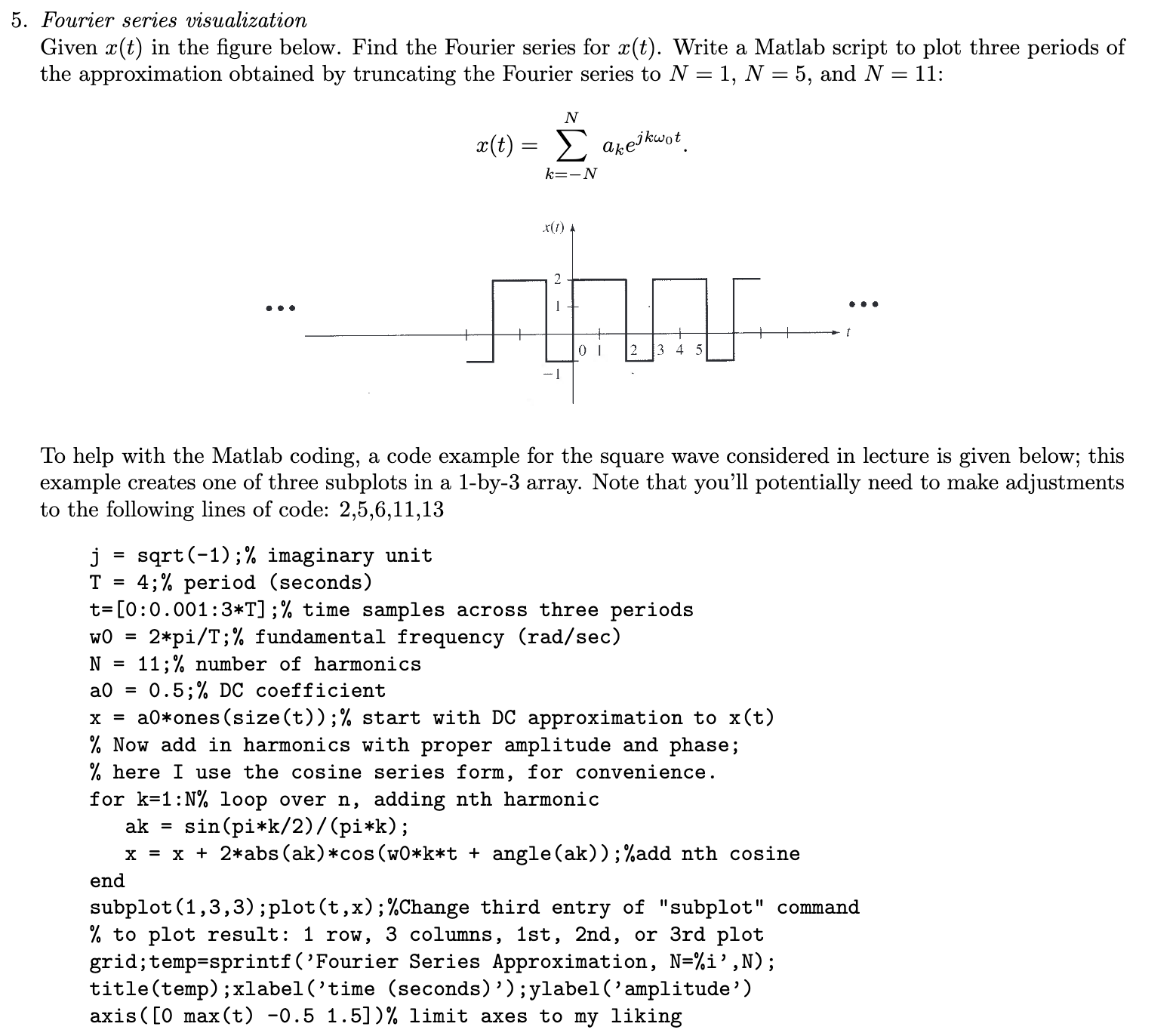
Fourier series visualization Given $x(t)$ in the figure below. Find the Fourier series for $x(t)$. Write a Matlab script to plot three periods of the approximation obtained by truncating the Fourier series to $N=1,N=5$, and $N=11$ : $x(t)={\sum }_{k=-N}^N{a}_k{e}^{jk{\omega }_{0}t}.$ To help with the Matlab coding, a code example for the square wave considered in lecture is given below; this example creates one of three subplots in a 1-by-3 array. Note that you'll potentially need to make adjustments to the following lines of code: $2,5,6,11,13$ $\mathrm{j}=\mathrm{sqrt}(-1);\%$ imaginary unit $\mathrm{T}=4;\%$ period (seconds) $\mathrm{t}=[0:0.001:3\ast \mathrm{T}];\%$ time samples across three periods w0 $=2\ast \mathrm{pi}/\mathrm{T};\%$ fundamental frequency ( $\mathrm{rad}/\sec$ ) $\mathrm{N}=11;\%$ number of harmonics $\mathrm{a}0=0.5;\%$ DC coefficient $\mathrm{x}=\mathrm{a}0\ast$ ones $(\mathrm{size}(\mathrm{t}));\%$ start with $\mathrm{DC}$ approximation to $\mathrm{x}(\mathrm{t})$ $\%$ Now add in harmonics with proper amplitude and phase; $\%$ here I use the cosine series form, for convenience. for $k=1:N\%$ loop over $n$, adding nth harmonic $\mathrm{ak}=\sin (\mathrm{pi}\ast \mathrm{k}/2)/(\mathrm{pi}\ast \mathrm{k});$ $\mathrm{x}=\mathrm{x}+2\ast \mathrm{abs}(\mathrm{ak})\ast \cos (\mathrm{w}0\ast \mathrm{k}\ast \mathrm{t}+\mathrm{angle}(\mathrm{ak}));\%$ add $\mathrm{nth}$ cosine end subplot $(1,3,3);plot(t,x);\%$ Change third entry of "subplot" command $\%$ to plot result: 1 row, 3 columns, 1st, 2nd, or 3rd plot grid;temp=sprintf ('Fourier Series Approximation, $\mathrm{N}=\%\mathrm{i}$ ', $\mathrm{N}$ ); title (temp); xlabel ('time (seconds)'); ylabel ('amplitude') $\mathrm{axis}([0\max (t)-\mathrm{0.51.5}])\%$ limit axes to my liking