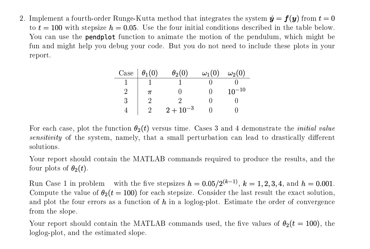
(Solved): Implement a fourth-order Runge-Kutta method that integrates the system y^()=f(y) from t=0 to t=10 ...

Implement a fourth-order Runge-Kutta method that integrates the system

from

to

with stepsize

. Use the four initial conditions described in the table below. You can use the pendplot function to animate the motion of the pendulum, which might be fun and might help you debug your code. But you do not need to include these plots in your report. For each case, plot the function

versus time. Cases 3 and 4 demonstrate the initial value sensitivity of the system, namely, that a small perturbation can lead to drastically different solutions. Your report should contain the MATLAB commands required to produce the results, and the four plots of

. Run Case 1 in problem

with the five stepsizes

, and

. Compute the value of

for each stepsize. Consider the last result the exact solution, and plot the four errors as a function of

in a loglog-plot. Estimate the order of convergence from the slope. Your report should contain the MATLAB commands used, the five values of

, the loglog-plot, and the estimated slope.