(Solved):   Use matlab to plot    Part B-2: Now let \( x(t) \) be a more complicated analog si ...

 

Use matlab to plot 

 

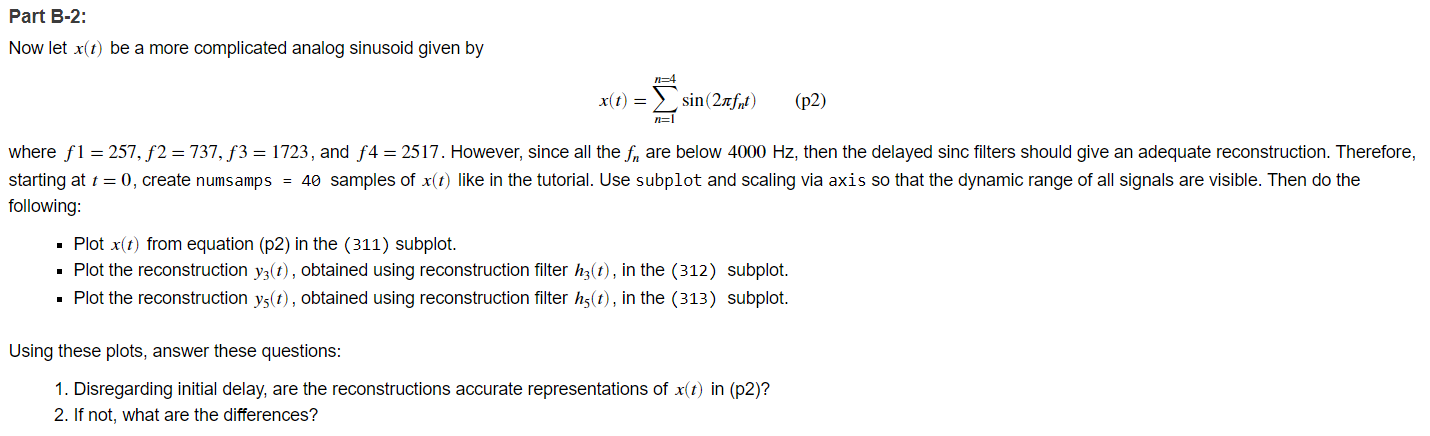
Part B-2: Now let \( x(t) \) be a more complicated analog sinusoid given by \[ x(t)=\sum_{n=1}^{n=4} \sin \left(2 \pi f_{n} t\right) \quad(\mathrm{p} 2) \] where \( f 1=257, f 2=737, f 3=1723 \), and \( f 4=2517 \). However, since all the \( f_{n} \) are below \( 4000 \mathrm{~Hz} \), then the delayed sinc filters should give an adequate reconstruction. Therefore, starting at \( t=0 \), create numsamps \( =40 \) samples of \( x(t) \) like in the tutorial. Use subplot and scaling via axis so that the dynamic range of all signals are the following: - Plot \( x(t) \) from equation (p2) in the (311) subplot. - Plot the reconstruction \( y_{3}(t) \), obtained using reconstruction filter \( h_{3}(t) \), in the (312) subplot. - Plot the reconstruction \( y_{5}(t) \), obtained using reconstruction filter \( h_{5}(t) \), in the (313) subplot. Using these plots, answer these questions: 1. Disregarding initial delay, are the reconstructions accurate representations of \( x(t) \) in (p2)? 2. If not, what are the differences?