(Solved): ..? Notes (1) As an illustration of these results we consider the case \( n ...

..?

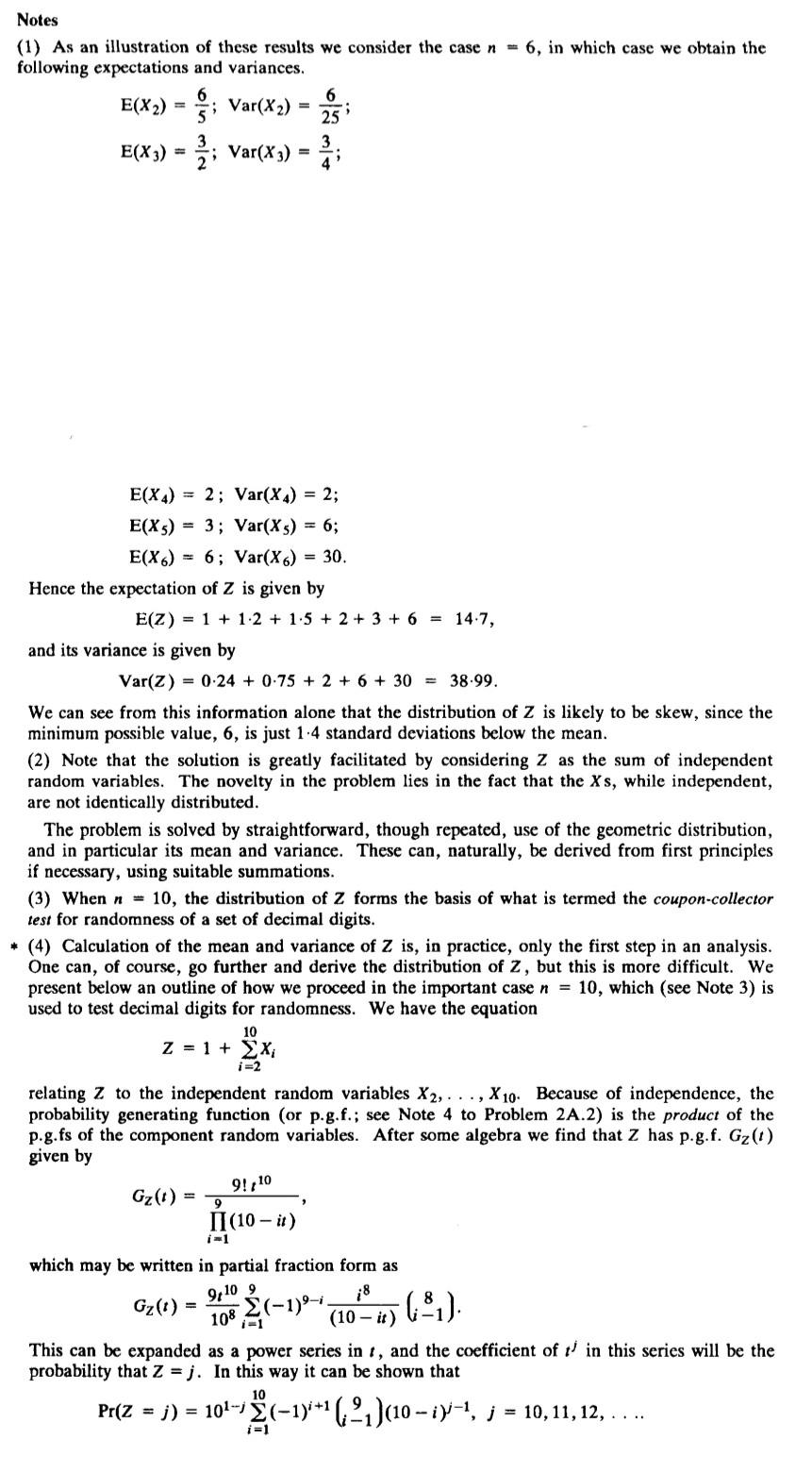
Notes (1) As an illustration of these results we consider the case \( n=6 \), in which case we obtain the following expectations and variances. \[ \begin{array}{l} \mathrm{E}\left(X_{2}\right)=\frac{6}{5} ; \operatorname{Var}\left(X_{2}\right)=\frac{6}{25} ; \\ \mathrm{E}\left(X_{3}\right)=\frac{3}{2} ; \operatorname{Var}\left(X_{3}\right)=\frac{3}{4} ; \end{array} \] \[ \begin{array}{l} \mathrm{E}\left(X_{4}\right)=2 ; \operatorname{Var}\left(X_{4}\right)=2 ; \\ \mathrm{E}\left(X_{5}\right)=3 ; \operatorname{Var}\left(X_{5}\right)=6 ; \\ \mathrm{E}\left(X_{6}\right)=6 ; \operatorname{Var}\left(X_{6}\right)=30 . \end{array} \] Hence the expectation of \( Z \) is given by \[ \mathrm{E}(Z)=1+1 \cdot 2+1 \cdot 5+2+3+6=14 \cdot 7 \text {, } \] and its variance is given by \[ \operatorname{Var}(Z)=0 \cdot 24+0.75+2+6+30=38.99 \text {. } \] We can see from this information alone that the distribution of \( Z \) is likely to be skew, since the minimum possible value, 6 , is just \( 1.4 \) standard deviations below the mean. (2) Note that the solution is greatly facilitated by considering \( z \) as the sum of independent random variables. The novelty in the problem lies in the fact that the \( X \mathrm{~s} \), while independent, are not identically distributed. The problem is solved by straightforward, though repeated, use of the geometric distribution, and in particular its mean and variance. These can, naturally, be derived from first principles if necessary, using suitable summations. (3) When \( n=10 \), the distribution of \( Z \) forms the basis of what is termed the coupon-collector test for randomness of a set of decimal digits. * (4) Calculation of the mean and variance of \( Z \) is, in practice, only the first step in an analysis. One can, of course, go further and derive the distribution of \( Z \), but this is more difficult. We present below an outline of how we proceed in the important case \( n=10 \), which (see Note 3 ) is used to test decimal digits for randomness. We have the equation \[ z=1+\sum_{i=2}^{10} x_{i} \] relating \( Z \) to the independent random variables \( X_{2}, \ldots, X_{10} \). Because of independence, the probability generating function (or p.g.f.; see Note 4 to Problem 2A.2) is the product of the p.g.fs of the component random variables. After some algebra we find that \( Z \) has p.g.f. \( G_{Z}(t) \) given by \[ G_{Z}(t)=\frac{9 ! t^{10}}{\prod_{i=1}^{9}(10-i t)} \] which may be written in partial fraction form as \[ G_{Z}(t)=\frac{9 t^{10}}{10^{8}} \sum_{i=1}^{9}(-1)^{9-i} \frac{i^{8}}{(10-i t)}\left(\begin{array}{c} 8 \\ i-1 \end{array}\right) \] This can be expanded as a power series in \( t \), and the coefficient of \( t^{j} \) in this series will be the probability that \( Z=j \). In this way it can be shown that \[ \operatorname{Pr}(Z=j)=10^{1-j} \sum_{i=1}^{10}(-1)^{i+1}\left(\begin{array}{c} 9 \\ i-1 \end{array}\right)(10-i)^{j-1}, j=10,11,12, \ldots . 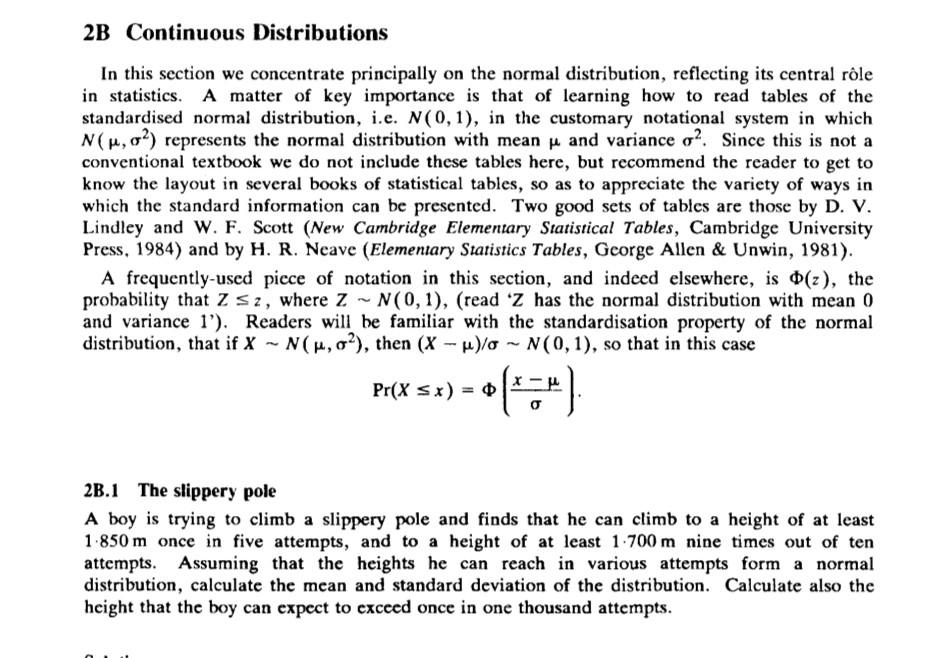\] 2B Continuous Distributions In this section we concentrate principally on the normal distribution, reflecting its central rôle in statistics. A matter of key importance is that of learning how to read tables of the standardised normal distribution, i.e. \( N(0,1) \), in the customary notational system in which \( N\left(\mu, \sigma^{2}\right) \) represents the normal distribution with mean \( \mu \) and variance \( \sigma^{2} \). Since this is not a conventional textbook we do not include these tables here, but recommend the reader to get to know the layout in several books of statistical tables, so as to appreciate the variety of ways in which the standard information can be presented. Two good sets of tables are those by \( \mathbf{D} \). V. Lindley and W. F. Scott (New Cambridge Elementary Statistical Tables, Cambridge University Press, 1984) and by H. R. Neave (Elementary Statistics Tables, Gcorge Allen \& Unwin, 1981). A frequently-used piece of notation in this section, and indeed elsewhere, is \( \Phi(z) \), the probability that \( Z \leq z \), where \( Z \sim N(0,1) \), (read ' \( Z \) has the normal distribution with mean 0 and variance 1'). Readers will be familiar with the standardisation property of the normal distribution, that if \( X \sim N\left(\mu, \sigma^{2}\right) \), then \( (X-\mu) / \sigma \sim N(0,1) \), so that in this case \[ \operatorname{Pr}(X \leq x)=\Phi\left(\frac{x-\mu}{\sigma}\right) \text {. } \] 2B.1 The slippery pole A boy is trying to climb a slippery pole and finds that he can climb to a height of at least \( 1.850 \mathrm{~m} \) once in five attempts, and to a height of at least \( 1.700 \mathrm{~m} \) nine times out of ten attempts. Assuming that the heights he can reach in various attempts form a normal distribution, calculate the mean and standard deviation of the distribution. Calculate also the height that the boy can expect to exceed once in one thousand attempts.