Home /
Expert Answers /
Statistics and Probability /
question-1-given-the-following-time-series-yt-its-acf-and-pacf-plots-are-as-follows-a-disc-pa399
(Solved): Question 1 Given the following time series yt : Its ACF and PACF plots are as follows: (a) Disc ...
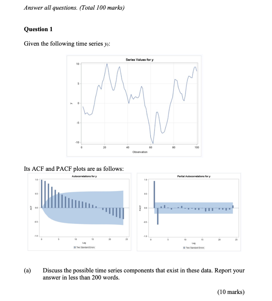
Question 1 Given the following time series : Its and plots are as follows: (a) Discuss the possible time series components that exist in these data. Report your answer in less than 200 words.
Expert Answer
Based on the given time series values and the ACF (Autocorrelation Function) and PACF (Partial Autocorrelation Function) plots, we can analyze the possible time series components that exist in the data.The ACF plot shows a significant autocorrelation at lag 1, which means that each observation is positively correlated with its immediate previous observation. This suggests the presence of a strong trend in the data. Additionally, there is a gradual decrease in autocorrelation as the lag increases, indicating a possible damping effect.The PACF plot displays a spike at lag 1, indicating a strong correlation between observations one period apart. This suggests the presence of an autoregressive (AR) component in the data.Considering these findings, the possible time series components that exist in the data are:1. Trend: The data exhibits a significant positive autocorrelation at lag 1, indicating a strong trend. This could be a linear or nonlinear trend contributing to the series's overall pattern.2. Damping: The gradual decrease in autocorrelation as the lag increases suggests a possible damping effect, indicating that the trend might not continue indefinitely but gradually diminish over time.3. Autoregressive (AR) Component: The spike in the PACF plot at lag 1 suggests the presence of an autoregressive component. This implies that the current observation is influenced by its immediate previous observation.Additional statistical techniques such as time series modeling (e.g., ARIMA, SARIMA) or decomposition methods (e.g., moving averages, exponential smoothing) can be applied to further analyze the time series components and their respective strengths.for plotting a graph use this steps ACF Plot: The ACF plot shows the autocorrelation values at different lags. Based on the information provided, the ACF plot should have a significant autocorrelation value at lag 1, and a gradual decrease in autocorrelation as the lag increases.PACF Plot: The PACF plot shows the partial autocorrelation values at different lags. According to the information given, there should be a spike at lag 1, indicating a strong correlation between observations one period apart.To interpret the plots:In the ACF plot, observe the values of autocorrelation at different lags. A significant autocorrelation at lag 1 suggests a strong trend, while a gradual decrease in autocorrelation indicates a possible damping effect.In the PACF plot, focus on the value at lag 1. A spike at lag 1 indicates a strong correlation between observations one period apart, implying the presence of an autoregressive component. decreasing graph decreasing graph as shown in the figure Based on the ACF and PACF plots, we can infer the following about the time series components in the data:1. Trend: The significant positive autocorrelation at lag 1 in the ACF plot indicates the presence of a strong trend. This means that each observation is positively correlated with its immediate previous observation, suggesting a consistent increase or decrease in the values over time. The trend can be linear or nonlinear.2. Damping: The gradual decrease in autocorrelation as the lag increases in the ACF plot suggests a possible damping effect. This means that the trend observed in the data may not continue indefinitely but rather diminish over time. The decreasing autocorrelation indicates a decreasing impact of past observations on future values.3. Autoregressive (AR) Component: The spike at lag 1 in the PACF plot suggests a strong correlation between observations one period apart. This indicates the presence of an autoregressive component. In other words, the current observation is influenced by its immediate previous observation, and the strength of this influence is captured by the spike in the PACF plot.To gain a more comprehensive understanding of the time series components and their strengths, additional statistical techniques such as time series modeling (e.g., ARIMA, SARIMA) or decomposition methods (e.g., moving averages, exponential smoothing) can be utilized. These techniques can provide further insights into the nature and characteristics of the trend, damping, and autoregressive components in the data.